electrical circuits 2: Characteristics of RLC circuits in Parallel Condition

Second-Order Solution

This page is going to talk about the solutions to a second-order, RLC circuit. The second-order solution is resonably complicated, and a complete understanding of it will require an understanding of differential equations. This book will not require you to know about differential equations, so we will describe the solutions without showing how to derive them. The derivations may be put into another chapter, eventually.

The aim of this chapter is to develop the complete response of the second-order circuit. There are a number of steps involved in determining the complete response:

Obtain the differential equations of the circuit
Determine the resonant frequency and the damping ratio
Obtain the characteristic equations of the circuit
Find the roots of the characteristic equation
Find the natural response
Find the forced response
Find the complete response

We will discuss all these steps one at a time.

[edit] Finding Differential Equations

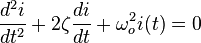
A Second-order circuit cannot possibly be solved until we obtain the second-order differential equation that describes the circuit. We will discuss here some of the techniques used for obtaining the second-order differential equation for an RLC Circuit.

Note: Parallel RLC Circuits are easier to solve in terms of current. Series RLC circuits are easier to solve in terms of voltage.

[edit] The Direct Method

The most direct method for finding the differential equations of a circuit is to perform a nodal analysis, or a mesh current analysis on the circuit, and then solve the equation for the input function. The final equation should only contain derivatives, no integrals.

[edit] The Variable Method

If we create 2 variables, g and h, we can use them to create a second-order differential equation. First, we set g and h to be either inductor currents, capacitor voltages, or both. Next, we create a single first order differential equation that has g = f(g, h). Then, we write another first-order differential equation that has the form:

$\frac{dh}{dt} = Kg$ or $\frac{1}{K}\frac{dh}{dt} = g$

Next, we substitute in our second equation into our first equation, and we have a second-order equation.

[edit] Zero-Input Response

The zero-input response of a circuit is the state of the circuit when there is no forcing function (no current input, and no voltage input). We can set the differential equation as such:

${{d^2 i} \over {dt^2}} + 2 \zeta {{di} \over {dt}} + \omega_o^2 i(t) = 0$

This gives rise to the characteristic equation of the circuit, which is explained below.

[edit] Characteristic Equation

The characteristic equation of an RLC circuit is obtained using the "Operator Method" described below, with zero input. The characteristic equation of an RLC circuit (series or parallel) will be:

$s^2i + {R \over L} si + {1 \over {LC}} i = 0$

The roots to the characteristic equation are the "solutions" that we are looking for.

[edit] Finding the Characteristic Equation

This method of obtaining the characteristic equation requires a little trickery. First, we create an operator s such that:

$sx = \frac{dx}{dt}$

Also, we can show higher-order operators as such:

$s^2x = \frac{d^2x}{dt^2}$

Where x is the voltage (in a series circuit) or the current (in a parellel circuit) of the circuit source. We write 2 first order differential equations for the inductor currents and/or the capacitor voltages in our circuit. We convert all the differentiations to s, and all the integrations (if any) into (1/s). We can then use Cramer's rule to solve for a solution.

[edit] Solutions

The solutions of the characteristic equation are given in terms of the resonant frequency and the damping ratio:

[Characteristic Equation Solution]

$s = - \zeta \pm \sqrt{\zeta^2 - \omega_o^2}$

If either of these two values are used for s in the assumed solution $x = A e s t$ and that solution completes the differential equation then it can be considered a valid solution. We will discuss this more, below.

[edit] Damping

The solutions to a circuit are dependant on the type of damping that the circuit exhibits, as determined by the relationship between the damping ratio and the resonant frequency. The different types of damping are Overdamping, Underdamping, and Critical Damping.

[edit] Overdamped

RLC series Over-Damped Response

A circuit is called Overdamped when the following condition is true:

α > ω 0

In this case, the solutions to the characteristic equation are two distinct, positive numbers, and are given by the equation:

$I(t)=A e^{\ s_1 t} + B e^{\ s_2 t}$ , where

$s_1,s_2 = - \alpha \pm \sqrt{\alpha^2 - \omega_0^2}$

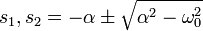
In a parallel circuit:

α = 1 / (2 R C)

ω 0 = 1 / s q r t (L C)

In a series circuit:

α = R / (2 L)

ω 0 = 1 / s q r t (L C)

Overdamped circuits are characterized as having a very large settling time, and possibly a large steady-state error.

[edit] Underdamped

A Circuit is called Underdamped when the damping ratio is less than the resonant frequency.

ζ < ω 0

In this case, the characteristic polynomial's solutions are complex conjugates. This results in oscillations or ringing in the circuit. The solution consists of two conjugate roots:

λ 1 = - ζ + i ω c

and

λ 2 = - ζ - i ω c

where

$\omega_c = \sqrt{\omega_o^2 - \zeta^2}$

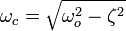
The solutions are:

$i(t) = Ae^{(-\zeta + i \omega_c)t} + Be^{(-\zeta - i \omega_c)t}$

for arbitrary constants A and B. Using Euler's formula, we can simplify the solution as:

$i(t)=e^{-\zeta t} \left[ C \sin(\omega_c t) + D \cos(\omega_c t) \right]$

for arbitrary constants C and D. These solutions are characterized by exponentially decaying sinusoidal response. The higher the Quality Factor (below), the longer it takes for the oscillations to decay.

[edit] Critically Damped

RLC series Critically Damped

A circuit is called Critically Damped if the damping factor is equal to the resonant frequency:

ζ = ω 0

In this case, the solutions to the characteristic equation is a double root. The two roots are identical ( $λ 1 = λ 2 = λ$ ), the solutions are:

I (t) = (A + B t) e λ t

for arbitrary constants A and B. Critically damped circuits typically have low overshoot, no oscillations, and quick settling time.

Parallel RLC

A parallel RLC Circuit.

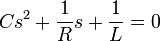
The differential equation to a parallel RLC circuit with a resistor R, a capacitor C, and an inductor L is as follows:

$C\frac{d^2v}{dt^2} + \frac{1}{R}\frac{dv}{dt} + {1 \over L}v = 0$

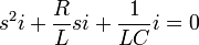
Where v is the voltage across the circuit. The characteristic equation then, is as follows:

$Cs^2 + {1 \over R}s + {1 \over L} = 0$

With the two roots:

$s_1 = -{1\over 2RC} + \sqrt{({1\over 2RC})^2 - {1 \over LC}}$

and

$s_2 = -{1\over 2RC} - \sqrt{({1\over 2RC})^2 - {1 \over LC}}$

[edit] Circuit Response

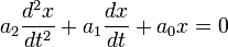
Once we have our differential equations, and our characteristic equations, we are ready to assemble the mathematical form of our circuit response. RLC Circuits have differential equations in the form:

$a_2 \frac{d^2x}{dt^2} + a_1\frac{dx}{dt} + a_0 x = f(t)$

Where f(t) is the forcing function of the RLC circuit.

[edit] Natural Response

The natural response of a circuit is the response of a given circuit to zero input (i.e. depending only upon the initial condition values). The natural Response to a circuit will be denoted as x_n(t). The natural response of the system must satisfy the unforced differential equation of the circuit:

[Unforced function]

$a_2 \frac{d^2x}{dt^2} + a_1\frac{dx}{dt} + a_0 x = 0$

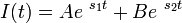
We remember this equation as being the "zero input response", that we discussed above. We now define the natural response to be an exponential function:

x n = A 1 e s t + A 2 e s t

Where s are the roots of the characteristic equation of the circuit. The reasons for choosing this specific solution for x_n is based in differential equations theory, and we will just accept it without proof for the time being. We can solve for the constant values, by using a system of two equations:

x (0) = A 1 + A 2

$\frac{dx(0)}{dt} = s_1A_1 + s_2A_2$

Where x is the voltage (of the elements in a parallel circuit) or the current (through the elements in a series circuit).

[edit] Forced Response

The forced response of a circuit is the way the circuit responds to an input forcing function. The Forced response is denoted as x_f(t).

Where the forced response must satisfy the forced differential equation:

[Forced function]

$a_2 \frac{d^2x}{dt^2} + a_1\frac{dx}{dt} + a_0 x = f(t)$

The forced response is based on the input function, so we can't give a general solution to it. However, we can provide a set of solutions for different inputs:

Input Form	Output Form
K (constant)	A (constant)
$M sin(ω t)$	$A sin(ω t) + B cos(ω t)$
$M e - a t$	$A e - a t$

[edit] Complete Response

The Complete response of a circuit is the sum of the forced response, and the natural response of the system:

[Complete Response]

x c (t) = x t (t) + x s (t)

Once we have derived the complete response of the circuit, we can say that we have "solved" the circuit, and are finished working.

Search This Blog

Tuesday, April 6, 2010

Characteristics of RLC circuits in Parallel Condition