electrical circuits 2: Concept of Impedance and Admittance

Complex impedance

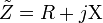
Impedance is represented as a complex quantity $\scriptstyle \tilde{Z}$ and the term complex impedance may be used interchangeably; the polar form conveniently captures both magnitude and phase characteristics,

$\tilde{Z} = Z e^{j\theta} \quad$

where the magnitude $\scriptstyle Z$ represents the ratio of the voltage difference amplitude to the current amplitude, while the argument $\scriptstyle \theta$ gives the phase difference between voltage and current and $\scriptstyle j$ is the imaginary unit. In Cartesian form,

$\tilde{Z} = R + j\Chi \quad$

where the real part of impedance is the resistance $\scriptstyle R$ and the imaginary part is the reactance $\scriptstyle \Chi$ .

Where it is required to add or subtract impedances the cartesian form is more convenient, but when quantities are multiplied or divided the calculation becomes simpler if the polar form is used. A circuit calculation, such as finding the total impedance of two impedances in parallel, may require conversion between forms several times during the calculation. Conversion between the forms follows the normal conversion rules of complex numbers.

[edit] Ohm's law

An AC supply applying a voltage $\scriptstyle V$ , across a load $\scriptstyle Z$ , driving a current $\scriptstyle I$ .

Main article: Ohm's law

The meaning of electrical impedance can be understood by substituting it into Ohm's law.^[4]^[5]

$\tilde{V} = \tilde{I}\tilde{Z} = \tilde{I} Z e^{j\theta} \quad$

The magnitude of the impedance $\scriptstyle Z$ acts just like resistance, giving the drop in voltage amplitude across an impedance $\scriptstyle \tilde{Z}$ for a given current $\scriptstyle \tilde{I}$ . The phase factor tells us that the current lags the voltage by a phase of $\scriptstyle \theta$ (i.e. in the time domain, the current signal is shifted $\scriptstyle \frac{\theta}{2 \pi} T$ to the right with respect to the voltage signal).^[6]

Just as impedance extends Ohm's law to cover AC circuits, other results from DC circuit analysis such as voltage division, current division, Thevenin's theorem, and Norton's theorem, can also be extended to AC circuits by replacing resistance with impedance.

[edit] Complex voltage and current

Generalized impedances in a circuit can be drawn with the same symbol as a resistor (US ANSI or DIN Euro) or with a labeled box.

In order to simplify calculations, sinusoidal voltage and current waves are commonly represented as complex-valued functions of time denoted as $\scriptstyle \tilde{V}$ and $\scriptstyle \tilde{I}$ .^[7]^[8]

$\ \tilde{V} = V_0e^{j(\omega t + \phi_V)}$

$\ \tilde{I} = I_0e^{j(\omega t + \phi_I)}$

Impedance is defined as the ratio of these quantities.

$\ \tilde{Z} = \frac{\tilde{V}}{\tilde{I}}$

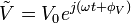
Substituting these into Ohm's law we have

$\begin{align} V_0e^{j(\omega t + \phi_V)} &= I_0e^{j(\omega t + \phi_I)} Z e^{j\theta} \\ &= I_0 Z e^{j(\omega t + \phi_I + \theta)} \end{align}$

Noting that this must hold for all $t$ , we may equate the magnitudes and phases to obtain

$\ V_0 = I_0 Z \quad$

$\ \phi_V = \phi_I + \theta \quad$

The magnitude equation is the familiar Ohm's law applied to the voltage and current amplitudes, while the second equation defines the phase relationship.

[edit] Validity of complex representation

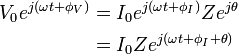
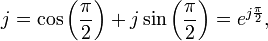
This representation using complex exponentials may be justified by noting that (by Euler's formula):

$\ \cos(\omega t + \phi) = \frac{1}{2} \Big[ e^{j(\omega t + \phi)} + e^{-j(\omega t + \phi)}\Big]$

i.e. a real-valued sinusoidal function (which may represent our voltage or current waveform) may be broken into two complex-valued functions. By the principle of superposition, we may analyse the behaviour of the sinusoid on the left-hand side by analysing the behaviour of the two complex terms on the right-hand side. Given the symmetry, we only need to perform the analysis for one right-hand term; the results will be identical for the other. At the end of any calculation, we may return to real-valued sinusoids by further noting that

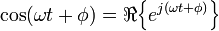
$\ \cos(\omega t + \phi) = \Re \Big\{ e^{j(\omega t + \phi)} \Big\}$

In other words, we simply take the real part of the result.

[edit] Phasors

Main article: Phasor (electronics)

A phasor is a constant complex number, usually expressed in exponential form, representing the complex amplitude (magnitude and phase) of a sinusoidal function of time. Phasors are used by electrical engineers to simplify computations involving sinusoids, where they can often reduce a differential equation problem to an algebraic one.

The impedance of a circuit element can be defined as the ratio of the phasor voltage across the element to the phasor current through the element, as determined by the relative amplitudes and phases of the voltage and current. This is identical to the definition from Ohm's law given above, recognising that the factors of $\scriptstyle e^{j\omega t}$ cancel.

[edit] Device examples

The phase angles in the equations for the impedance of inductors and capacitors indicate that the voltage across a capacitor lags the current through it by a phase of

π / 2

, while the voltage across an inductor leads the current through it by

π / 2

. The identical voltage and current amplitudes tell us that the magnitude of the impedance is equal to one.

The impedance of an ideal resistor is purely real and is referred to as a resistive impedance:

$\tilde{Z}_R = R.$

Ideal inductors and capacitors have a purely imaginary reactive impedance:

$\tilde{Z}_L = j\omega L,$

$\tilde{Z}_C = \frac{1}{j\omega C} \, .$

Note the following identities for the imaginary unit and its reciprocal:

$j = \cos{\left(\frac{\pi}{2}\right)} + j\sin{\left(\frac{\pi}{2}\right)} = e^{j\frac{\pi}{2}},$

$\frac{1}{j} = -j = \cos{\left(-\frac{\pi}{2}\right)} + j\sin{\left(-\frac{\pi}{2}\right)} = e^{j(-\frac{\pi}{2})}.$

Thus we can rewrite the inductor and capacitor impedance equations in polar form:

$\tilde{Z}_L = \omega Le^{j\frac{\pi}{2}},$

$\tilde{Z}_C = \frac{1}{\omega C}e^{j(-\frac{\pi}{2})}.$

The magnitude tells us the change in voltage amplitude for a given current amplitude through our impedance, while the exponential factors give the phase relationship.

[edit] Deriving the device specific impedances

What follows below is a derivation of impedance for each of the three basic circuit elements, the resistor, the capacitor, and the inductor. Although the idea can be extended to define the relationship between the voltage and current of any arbitrary signal, these derivations will assume sinusoidal signals, since any arbitrary signal can be approximated as a sum of sinusoids through Fourier Analysis.

[edit] Resistor

For a resistor, we have the relation:

$v_{\text{R}} \left( t \right) = {i_{\text{R}} \left( t \right)}R.$

This is simply a statement of Ohm's Law.

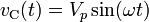
Considering the voltage signal to be

$v_{\text{R}}(t) = V_p \sin(\omega t) \, ,$

it follows that

$\frac{v_{\text{R}} \left( t \right)}{i_{\text{R}} \left( t \right)} = \frac{V_p \sin(\omega t)}{I_p \sin \left( \omega t \right)} = R.$

This tells us that the ratio of AC voltage amplitude to AC current amplitude across a resistor is $\scriptstyle R$ , and that the AC voltage leads the AC current across a resistor by 0 degrees.

This result is commonly expressed as

$Z_{\text{resistor}} = R \, .$

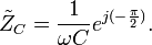
[edit] Capacitor

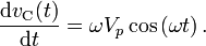
For a capacitor, we have the relation:

$i_{\text{C}}(t) = C \frac{\operatorname{d}v_{\text{C}}(t)}{\operatorname{d}t}.$

Considering the voltage signal to be

$v_{\text{C}}(t) = V_p \sin(\omega t) \,$

it follows that

$\frac{\operatorname{d}v_{\text{C}}(t)}{\operatorname{d}t} = \omega V_p \cos \left( \omega t \right).$

And thus

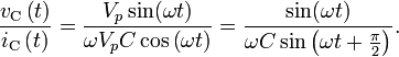
$\frac{v_{\text{C}} \left( t \right)}{i_{\text{C}} \left( t \right)} = \frac{V_p \sin(\omega t)}{\omega V_p C \cos \left( \omega t \right)}= \frac{\sin(\omega t)}{\omega C \sin \left( \omega t + \frac{\pi}{2}\right)}.$

This tells us that the ratio of AC voltage amplitude to AC current amplitude across a capacitor is $\scriptstyle \frac{1}{\omega C}$ , and that the AC voltage leads the AC current across a capacitor by -90 degrees (or the AC current leads the AC voltage across a capacitor by 90 degrees).

This result is commonly expressed in polar form, as

$\tilde{Z}_{\text{capacitor}} = \frac{1}{\omega C} e^{-j \frac{\pi}{2}}$

or, by applying Euler's formula, as

$\tilde{Z}_{\text{capacitor}} = -j\frac{1}{\omega C} = \frac{1}{j \omega C} \, .$

[edit] Inductor

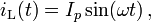
For the inductor, we have the relation:

$v_{\text{L}}(t) = L \frac{\operatorname{d}i_{\text{L}}(t)}{\operatorname{d}t}.$

This time, considering the current signal to be

$i_{\text{L}}(t) = I_p \sin(\omega t) \, ,$

it follows that

$\frac{\operatorname{d}i_{\text{L}}(t)}{\operatorname{d}t} = \omega I_p \cos \left( \omega t \right).$

And thus

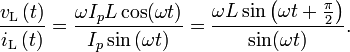
$\frac{v_{\text{L}} \left( t \right)}{i_{\text{L}} \left( t \right)} = \frac{\omega I_p L \cos(\omega t)}{I_p \sin \left( \omega t \right)}= \frac{\omega L \sin \left( \omega t + \frac{\pi}{2}\right)}{\sin(\omega t)}.$

This tells us that the ratio of AC voltage amplitude to AC current amplitude across an inductor is $\scriptstyle \omega L$ , and that the AC voltage leads the AC current across an inductor by 90 degrees.

This result is commonly expressed in polar form, as

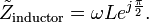
$\tilde{Z}_{\text{inductor}} = \omega L e^{j \frac{\pi}{2}} .$

Or, more simply, using Euler's formula, as

$\tilde{Z}_{\text{inductor}} = j \omega L. \,$

[edit] Resistance vs reactance

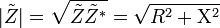
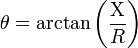
It is important to realize that resistance and reactance are not individually significant; together they determine the magnitude and phase of the impedance, through the following relations:

$|\tilde{Z}| = \sqrt{\tilde{Z}\tilde{Z}^*} = \sqrt{R^2 + \Chi^2}$

$\theta = \arctan{\left(\frac{\Chi}{R}\right)}$

In many applications the relative phase of the voltage and current is not critical so only the magnitude of the impedance is significant.

[edit] Resistance

Main article: Electrical resistance

Resistance $\scriptstyle R$ is the real part of impedance; a device with a purely resistive impedance exhibits no phase shift between the voltage and current.

$R = Z \cos{\theta} \quad$

[edit] Reactance

Main article: Electrical reactance

Reactance $\scriptstyle \Chi$ is the imaginary part of the impedance; a component with a finite reactance induces a phase shift $\scriptstyle \theta$ between the voltage across it and the current through it.

$\Chi = Z \sin{\theta} \quad$

A purely reactive component is distinguished by the fact that the sinusoidal voltage across the component is in quadrature with the sinusoidal current through the component. This implies that the component alternately absorbs energy from the circuit and then returns energy to the circuit. A pure reactance will not dissipate any power.

[edit] Capacitive reactance

Main article: Capacitor

A capacitor has a purely reactive impedance which is inversely proportional to the signal frequency. A capacitor consists of two conductors separated by an insulator, also known as a dielectric.

At low frequencies a capacitor is open circuit, as no charge flows in the dielectric. A DC voltage applied across a capacitor causes charge to accumulate on one side; the electric field due to the accumulated charge is the source of the opposition to the current. When the potential associated with the charge exactly balances the applied voltage, the current goes to zero.

Driven by an AC supply, a capacitor will only accumulate a limited amount of charge before the potential difference changes sign and the charge dissipates. The higher the frequency, the less charge will accumulate and the smaller the opposition to the current.

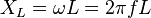
[edit] Inductive reactance

Main article: Inductance

Inductive reactance $\scriptstyle{X_L}$ is proportional to the signal frequency $\scriptstyle{f}$ and the inductance $\scriptstyle{L}$ .

$X_L = \omega L = 2\pi f L\quad$

An inductor consists of a coiled conductor. Faraday's law of electromagnetic induction gives the back emf $\scriptstyle{\mathcal{E}}$ (voltage opposing current) due to a rate-of-change of magnetic flux density $\scriptstyle{B}$ through a current loop.

$\mathcal{E} = -{{d\Phi_B} \over dt}\quad$

For an inductor consisting of a coil with $N$ loops this gives.

$\mathcal{E} = -N{d\Phi_B \over dt}\quad$

The back-emf is the source of the opposition to current flow. A constant direct current has a zero rate-of-change, and sees an inductor as a short-circuit (it is typically made from a material with a low resistivity). An alternating current has a time-averaged rate-of-change that is proportional to frequency, this causes the increase in inductive reactance with frequency.

[edit] Combining impedances

Main article: Series and parallel circuits

The total impedance of many simple networks of components can be calculated using the rules for combining impedances in series and parallel. The rules are identical to those used for combining resistances, except that the numbers in general will be complex numbers. In the general case however, equivalent impedance transforms in addition to series and parallel will be required.

[edit] Series combination

For components connected in series, the current through each circuit element is the same; the total impedance is simply the sum of the component impedances.

$\tilde{Z}_{\text{eq}} = \tilde{Z}_1 + \tilde{Z}_2 + ... + \tilde{Z}_n \quad$

Or explicitly in real and imaginary terms:

$\tilde{Z}_{\text{eq}} = R + j\Chi = (R_1 + R_2 + ... + R_n) + j(\Chi_1 + \Chi_2 + ... + \Chi_n) \quad$

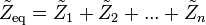
[edit] Parallel combination

For components connected in parallel, the voltage across each circuit element is the same; the ratio of currents through any two elements is the inverse ratio of their impedances.

Hence the inverse total impedance is the sum of the inverses of the component impedances:

$\frac{1}{\tilde{Z}_{\text{eq}}} = \frac{1}{\tilde{Z}_1} + \frac{1}{\tilde{Z}_2} +.. + \frac{1}{\tilde{Z}_n}\,$

or, when n = 2:

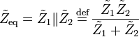
$\tilde{Z}_{\text{eq}} = \tilde{Z}_1 \| \tilde{Z}_2 \,\stackrel{\text{def}}{=}\, \frac{\tilde{Z}_1 \tilde{Z}_2}{\tilde{Z}_1 + \tilde{Z}_2} \quad$

The equivalent impedance $\scriptstyle \tilde{Z}_{\text{eq}}$ can be calculated in terms of the equivalent resistance $\scriptstyle R_{\text{eq}}$ and reactance $\scriptstyle \Chi_{\text{eq}}$ .^[9]

$\tilde{Z}_{\text{eq}} = R_{\text{eq}} + j \Chi_{\text{eq}} \quad$

$R_{\text{eq}} = \frac{(\Chi_1 R_2 + \Chi_2 R_1) (\Chi_1 + \Chi_2) + (R_1 R_2 - \Chi_1 \Chi_2) (R_1 + R_2)}{(R_1 + R_2)^2 + (\Chi_1 + \Chi_2)^2}$

$\Chi_{\text{eq}} = \frac{(\Chi_1 R_2 + \Chi_2 R_1) (R_1 + R_2) - (R_1 R_2 - \Chi_1 \Chi_2) (\Chi_1 + \Chi_2)}{(R_1 + R_2)^2 + (\Chi_1 + \Chi_2)^2}$

[edit] Measuring Impedance

According to Ohm’s law the impedance of a device can be calculated by complex division of the voltage and current. The impedance of the device can be calculated by applying a sinusoidal voltage to the device in series with a resistor, and measuring the voltage across the resistor and across the device. Performing this measurement by sweeping the frequencies of the applied signal provides the impedance phase and magnitude.^[10]

[edit] Impulse impedance spectroscopy

The use of an impulse response may be used in combination with the fast Fourier transform (FFT) to rapidly measure the electrical impedance of various electrical devices. The technique compares well to other methodologies such as network and impedance analyzers while providing additional versatility in the electrical impedance measurement. The technique is theoretically simple, easy to implement and completed with ordinary laboratory instrumentation for minimal cost.^[10]

[edit] Variable impedance

In general, neither impedance nor admittance can be time varying as they are defined for complex exponentials for –∞ < t < +∞. If the complex exponential voltage–current ratio changes over time or amplitude, the circuit element cannot be described using the frequency domain. However, many systems (e.g., varicaps that are used in radio tuners) may exhibit non-linear or time-varying voltage–current ratios that appear to be LTI for small signals over small observation windows; hence, they can be roughly described as having a time-varying impedance. That is, this description is an approximation; over large signal swings or observation windows, the voltage–current relationship is non-LTI and cannot be described by impedance.

In electrical engineering, the admittance (Y) is the inverse of the impedance (Z). The SI unit of admittance is the siemens (symbol S). Oliver Heaviside coined the term in December 1887.^[1]

$Y = Z^{-1} = 1/Z \,$

where

Y is the admittance, measured in siemens

Z is the impedance, measured in ohms

Note that the synonymous unit mho, and the symbol ℧ (an upside-down uppercase omega Ω), are also in common use.

Admittance is a measure of how easily a circuit or device will allow a current to flow. Resistance is a measure of the opposition of a circuit to the flow of a steady current, while impedance takes into account not only the resistance but also dynamic effects (known as reactance). Likewise, admittance is not only a measure of the ease with which a steady current can flow (conductance, G, the inverse of resistance), but also the dynamic effects of susceptance, B, (the inverse of reactance):

$Y = G + j B \,$

[hide]

[edit] Conversion from impedance to admittance

Parts of this article or section rely on the reader's knowledge of the complex impedance representation of capacitors and inductors and on knowledge of the frequency domain representation of signals.

The impedance, Z, is composed of real and imaginary parts,

$Z = R + jX \,$

where

R is the resistance, measured in ohms

X is the reactance, measured in ohms

$Y = Z^{-1}= \frac{1}{R+jX} = \left( \frac{R}{R^2+X^2} \right) + j\left(\frac{-X}{R^2+X^2}\right)$

Admittance, just like impedance, is a complex number, made up of a real part (the conductance, G), and an imaginary part (the susceptance, B), thus:

$Y = G + jB \,\!$ ,

where G (conductance) and B (susceptance) are given by:

$G = \Re(Y) = \left( \frac{R}{R^2+X^2} \right)$

$B = \Im(Y) = \left( \frac{-X}{R^2+X^2}\right)$

The magnitude and phase of the admittance are given by:

$\left | Y \right | = \sqrt {G^2 + B^2} = \frac {1} {\sqrt {R^2 + X^2} } \,$

$\angle Y = \arctan \left( {\frac{B}{G}} \right)= \arctan \left( {\frac{-X}{R}} \right)$

where

G is the conductance, measured in siemens

B is the susceptance, also measured in siemens

Note that (as shown above) the signs of reactances become reversed in the admittance domain, i.e. capactive susceptance is positive and inductive suceptance is negative.

[edit] Admittance in mechanics

In mechanical systems (particularly in the field of haptics), an admittance is a dynamic mapping from force to motion. In other words, an equation (or virtual environment) describing an admittance would have inputs of force and would have outputs such as position or velocity. So, an admittance device would sense the input force and "admit" a certain amount of motion.

Similar to the electrical meanings of admittance and impedance, an impedance in the mechanical sense can be thought of as the "inverse" of admittance. That is, it is a dynamic mapping from motion to force. An impedance device would sense the input motion and "impede" the motion with some force.

An example of these concepts is a virtual spring. The equation describing a spring is Hooke's Law,

$F = -kx \,$

If the input to the virtual spring is the spring displacement, x, and the output is the force that the virtual spring applies, F, then the virtual spring would be classified as an impedance. If the input to the virtual spring is the force applied to the spring, F, and the output is the spring displacement, x, then the virtual spring would be classified as an admittance.

[edit] Admittance in geophysics

The geophysical conception of admittance is similar to that described above for mechanical systems. The concept is primarily used for describing the small effects of atmospheric pressure on earth gravity. Studies have also been carried out regarding the gravity of Venus.^[2] Admittance in geophysics takes atmospheric pressure as the input and measures small changes in the gravitational field as the output. Geophysics admittance is commonly measured in μGal/mbar. These units convert according to 1 Gal = 0.01 m/s² and 1 bar = 100 kPa, so in SI units the measurement would be in units of;

$\frac{\mathrm{m}/\mathrm{s}^2}{\mathrm{Pa}}$ or $\frac{\mathrm{m}/\mathrm{s}^2}{\mathrm{N}/\mathrm{m}^2}$ or $\frac{\mathrm{m}^3}{\mathrm{N}\cdot \mathrm{s}^2}$ or, in primary units $\frac{\mathrm{m}^2}{\mathrm{kg}}$

However, the relationship is not a straightforward one of proportionality. Rather, an admittance function is described which is time and frequency dependent in a complex way.^[3]

Search This Blog

Tuesday, April 6, 2010

Concept of Impedance and Admittance

Complex impedance

[edit] Ohm's law

[edit] Complex voltage and current

[edit] Validity of complex representation

[edit] Phasors

[edit] Device examples

[edit] Deriving the device specific impedances

[edit] Resistor

[edit] Capacitor

[edit] Inductor

[edit] Resistance vs reactance

[edit] Resistance

[edit] Reactance

[edit] Capacitive reactance

[edit] Inductive reactance

[edit] Combining impedances

[edit] Series combination

[edit] Parallel combination

[edit] Measuring Impedance

[edit] Impulse impedance spectroscopy

[edit] Variable impedance

Contents

[edit] Conversion from impedance to admittance

[edit] Admittance in mechanics

[edit] Admittance in geophysics

No comments:

Post a Comment

electrical circuits 2

WEEK

Followers

Blog Archive

About Me